Analyzing Top 10.000 Most Popular Movies on IMDB

Finding the common characteristics among Top 10.000 movies of all time

Author

invictus

EDA with R

Setup

Library

library(tidyverse)

── Attaching core tidyverse packages ──────────────────────── tidyverse 2.0.0 ──
✔ dplyr     1.1.4     ✔ readr     2.1.5
✔ forcats   1.0.0     ✔ stringr   1.5.1
✔ ggplot2   3.5.1     ✔ tibble    3.2.1
✔ lubridate 1.9.3     ✔ tidyr     1.3.1
✔ purrr     1.0.2     
── Conflicts ────────────────────────────────────────── tidyverse_conflicts() ──
✖ dplyr::filter() masks stats::filter()
✖ dplyr::lag()    masks stats::lag()
ℹ Use the conflicted package (<http://conflicted.r-lib.org/>) to force all conflicts to become errors

library(naniar)
library(summarytools)

Warning: no DISPLAY variable so Tk is not available

system might not have X11 capabilities; in case of errors when using dfSummary(), set st_options(use.x11 = FALSE)

Attaching package: 'summarytools'

The following object is masked from 'package:tibble':

    view

library(janitor)


Attaching package: 'janitor'

The following objects are masked from 'package:stats':

    chisq.test, fisher.test

library(DataExplorer)
library(scales)


Attaching package: 'scales'

The following object is masked from 'package:purrr':

    discard

The following object is masked from 'package:readr':

    col_factor

Options

update_geom_defaults("bar", list(fill = 'grey', color = 'black'))

Dataset

df <- read_csv('top_10_000_movies.csv', na = '\\N')

Rows: 10000 Columns: 7
── Column specification ────────────────────────────────────────────────────────
Delimiter: ","
chr (3): tconst, primaryTitle, genres
dbl (4): startYear, runtimeMinutes, averageRating, numVotes

ℹ Use `spec()` to retrieve the full column specification for this data.
ℹ Specify the column types or set `show_col_types = FALSE` to quiet this message.

Clean Data

df

# A tibble: 10,000 × 7
   tconst    primaryTitle genres startYear runtimeMinutes averageRating numVotes
   <chr>     <chr>        <chr>      <dbl>          <dbl>         <dbl>    <dbl>
 1 tt0111161 The Shawsha… Drama       1994            142           9.3  2933616
 2 tt0468569 The Dark Kn… Actio…      2008            152           9    2914022
 3 tt1375666 Inception    Actio…      2010            148           8.8  2587592
 4 tt0137523 Fight Club   Drama       1999            139           8.8  2365113
 5 tt0109830 Forrest Gump Drama…      1994            142           8.8  2294287
 6 tt0110912 Pulp Fiction Crime…      1994            154           8.9  2253218
 7 tt0816692 Interstellar Adven…      2014            169           8.7  2149979
 8 tt0133093 The Matrix   Actio…      1999            136           8.7  2083320
 9 tt0068646 The Godfath… Crime…      1972            175           9.2  2044687
10 tt0120737 The Lord of… Actio…      2001            178           8.9  2035850
# ℹ 9,990 more rows

Check Missing Data

df |> 
  vis_miss()

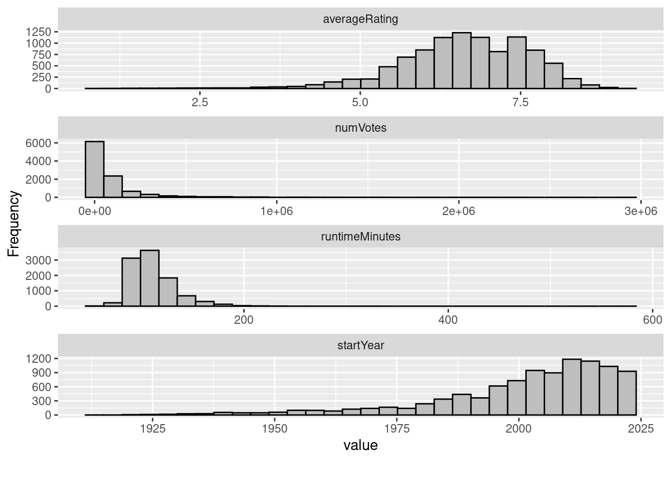
Check Numeric Distribution

Overall

df |> 
  plot_histogram(ncol = 1)

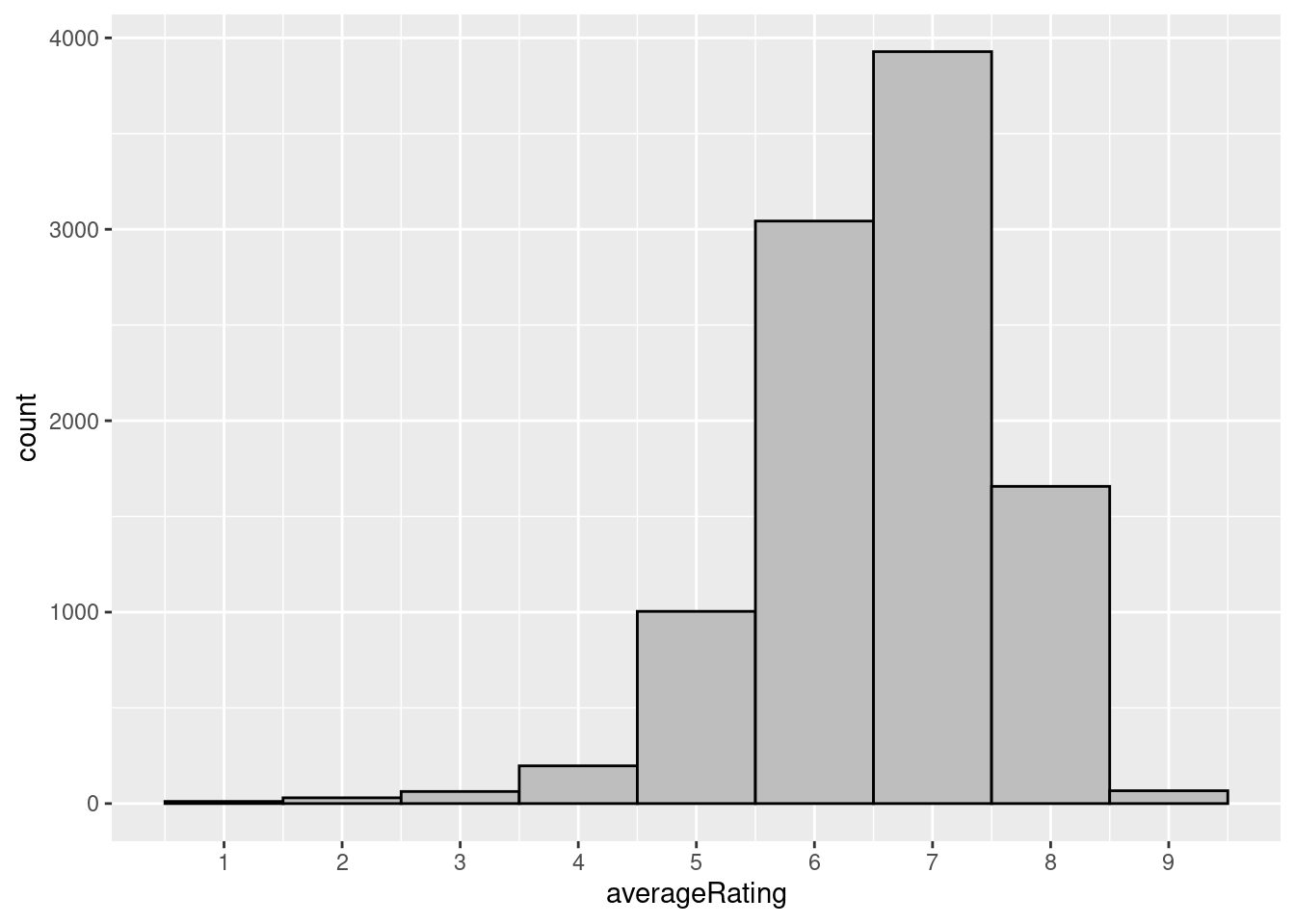
Average Rating

df |> 
  ggplot(aes(averageRating)) +
  geom_histogram(binwidth = 1) +
  scale_x_continuous(breaks = seq(0,10,1))

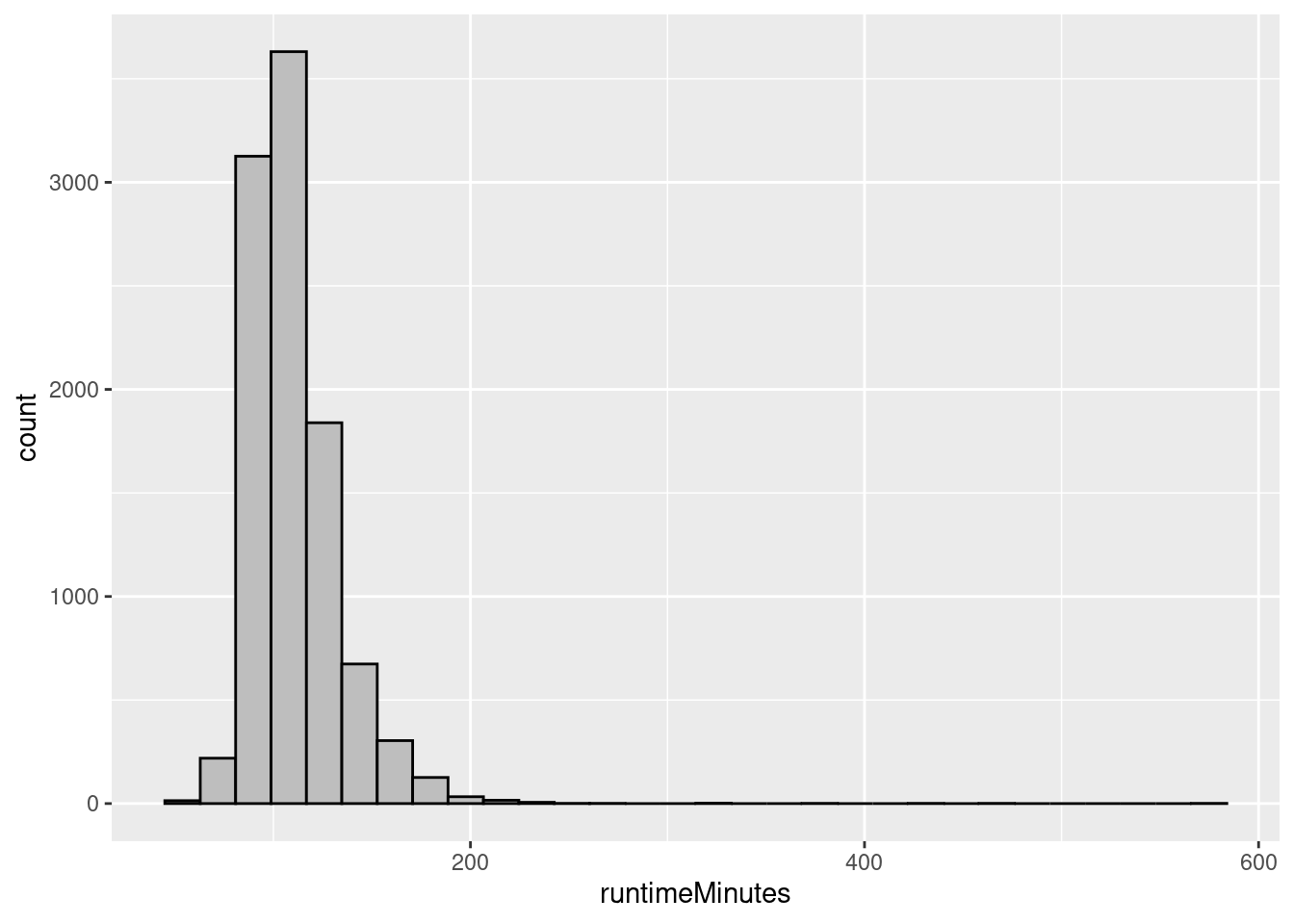
Runtime Minutes

df |> 
  ggplot(aes(runtimeMinutes)) +
  geom_histogram()

`stat_bin()` using `bins = 30`. Pick better value with `binwidth`.

Warning: Removed 4 rows containing non-finite outside the scale range
(`stat_bin()`).

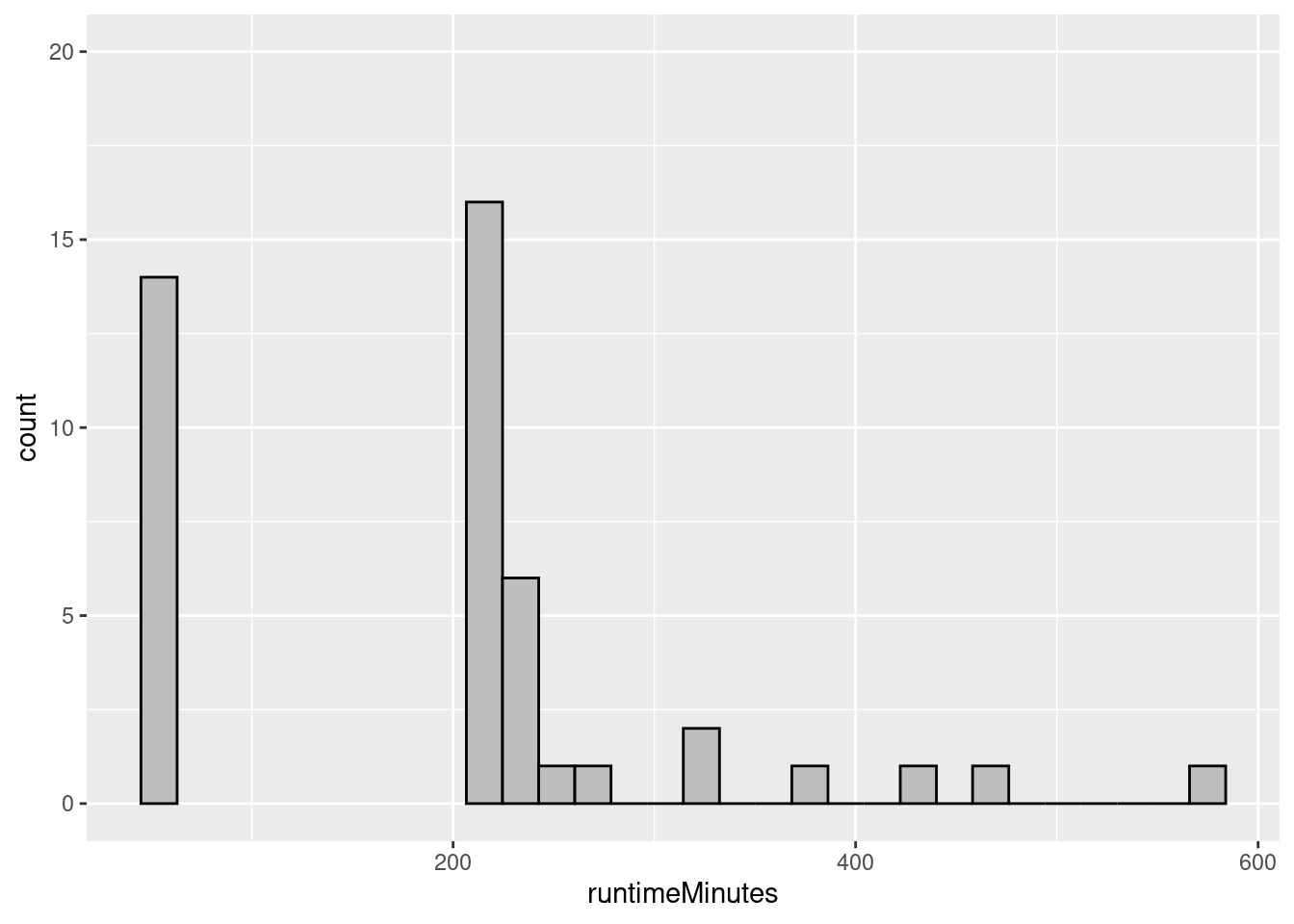
df |> 
  ggplot(aes(runtimeMinutes)) +
  geom_histogram() +
  ylim(0,20)

`stat_bin()` using `bins = 30`. Pick better value with `binwidth`.

Warning: Removed 4 rows containing non-finite outside the scale range
(`stat_bin()`).

Warning: Removed 8 rows containing missing values or values outside the scale range
(`geom_bar()`).

Num Votes

df |> 
  pull(numVotes) |> 
  cut(breaks = seq(1, 3000000, 100000), dig.lab = 50, right = FALSE, include.lowest = TRUE) |> 
  tabyl() |> 
  as.tibble() |> 
  rename(range = 1) |> 
  mutate(percent = label_percent(accuracy=0.001)(percent)) |> 
  select(-valid_percent)

Warning: `as.tibble()` was deprecated in tibble 2.0.0.
ℹ Please use `as_tibble()` instead.
ℹ The signature and semantics have changed, see `?as_tibble`.

# A tibble: 30 × 3
   range                n percent
   <fct>            <int> <chr>  
 1 [1,100001)        7749 77.490%
 2 [100001,200001)   1130 11.300%
 3 [200001,300001)    470 4.700% 
 4 [300001,400001)    209 2.090% 
 5 [400001,500001)    131 1.310% 
 6 [500001,600001)     73 0.730% 
 7 [600001,700001)     62 0.620% 
 8 [700001,800001)     50 0.500% 
 9 [800001,900001)     37 0.370% 
10 [900001,1000001)    21 0.210% 
# ℹ 20 more rows

  # mutate(percent = label_percent(accuracy=0.01)(percent))
  # mutate(range = format(range, big.mark = ','))

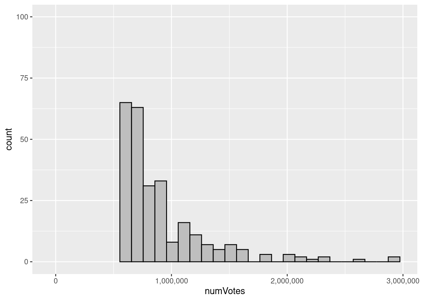
df |> 
  ggplot(aes(numVotes)) +
  geom_histogram() +
  ylim(c(0, 100)) +
  scale_x_continuous(labels = comma)

`stat_bin()` using `bins = 30`. Pick better value with `binwidth`.

Warning: Removed 6 rows containing missing values or values outside the scale range
(`geom_bar()`).

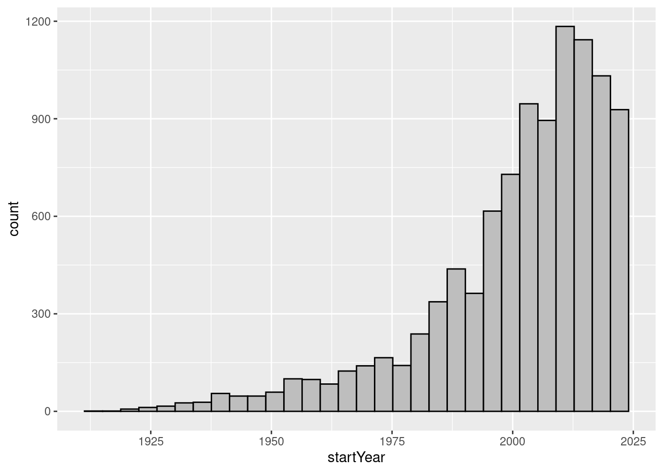
df |> 
  ggplot(aes(startYear)) +
  geom_histogram()

`stat_bin()` using `bins = 30`. Pick better value with `binwidth`.

Genre

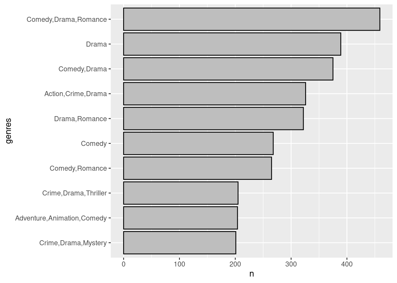
df <- df |> 
  mutate(genres = fct_rev(fct_infreq(genres)))

df |> 
  count(genres) |> 
  arrange(desc(n)) |>
  slice_head(n = 10) |> 
  ggplot(aes(n, genres)) +
  geom_col()

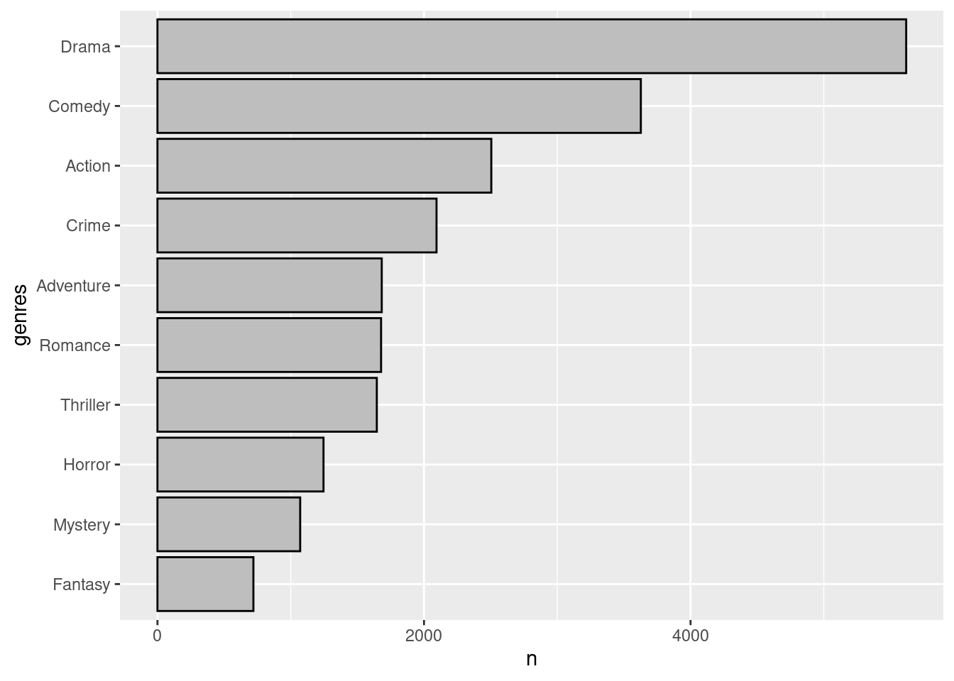
df_unnested_genre <- df |> 
  mutate(genres = str_split(genres, ',')) |> 
  unnest_longer(genres) |> 
  mutate(genres = fct_rev(fct_infreq(genres)))

df_unnested_genre |> 
  count(genres) |> 
  arrange(desc(n)) |> 
  slice_head(n = 10) |> 
  ggplot(aes(genres, n)) +
  geom_col() +
  coord_flip()

Analyze Data

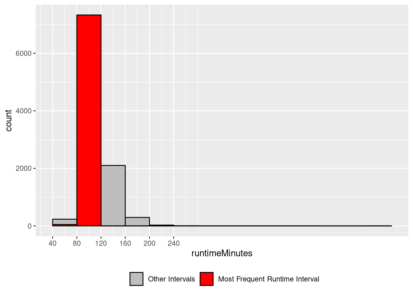
Most Common Runtime Range

df |> 
  ggplot(aes(runtimeMinutes)) +
  geom_histogram(aes(fill = runtimeMinutes >= 80 & runtimeMinutes <= 120), 
                 binwidth = 40, boundary = 0) +
  scale_x_continuous(breaks = seq(0, 240, 40)) +
  scale_fill_manual(values = c("FALSE" = "grey", "TRUE" = "red"),
                    labels = c("FALSE" = "Other Intervals", "TRUE" = "Most Frequent Runtime Interval")) +
  labs(fill = "") +
  theme(legend.position = "bottom")

Warning: Removed 4 rows containing non-finite outside the scale range
(`stat_bin()`).

df |> 
  pull(runtimeMinutes) |> 
  cut(breaks = seq(1, 600, 40), dig.lab = 50) |> 
  tabyl() |> 
  as.tibble() |> 
  rename(range = 1) |> 
  mutate(percent = label_percent(accuracy=0.01)(percent)) |> 
  select(-valid_percent)

# A tibble: 15 × 3
   range         n percent
   <fct>     <int> <chr>  
 1 (1,41]        0 0.00%  
 2 (41,81]     281 2.81%  
 3 (81,121]   7393 73.93% 
 4 (121,161]  2006 20.06% 
 5 (161,201]   280 2.80%  
 6 (201,241]    26 0.26%  
 7 (241,281]     4 0.04%  
 8 (281,321]     2 0.02%  
 9 (321,361]     0 0.00%  
10 (361,401]     1 0.01%  
11 (401,441]     1 0.01%  
12 (441,481]     1 0.01%  
13 (481,521]     0 0.00%  
14 (521,561]     0 0.00%  
15 <NA>          5 0.05%

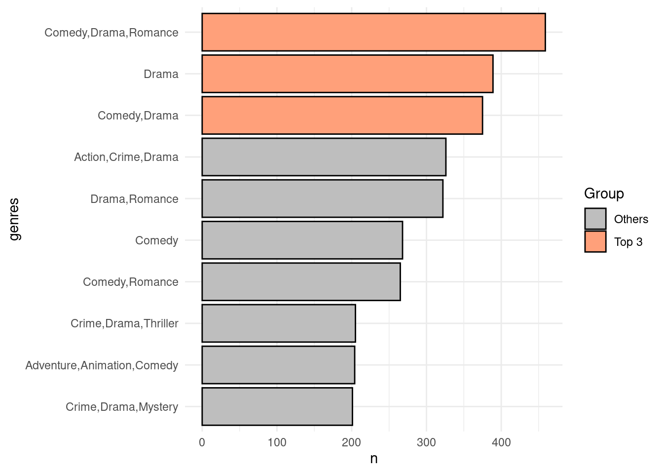
Most Common Genre Combinations

df |> 
  count(genres) |> 
  arrange(desc(n)) |>
  mutate(is_top3 = ifelse(row_number() <= 3, "Top 3", "Others")) |>  # Flag top 5
  slice_head(n = 10) |> 
  ggplot(aes(n, genres, fill = is_top3)) +  # Use fill aesthetic to differentiate
  geom_col() +
  scale_fill_manual(values = c("Top 3" = "#FFA07A", "Others" = "grey")) +  # Highlight top 5
  theme_minimal() +
  labs(fill = "Group")  # Add legend

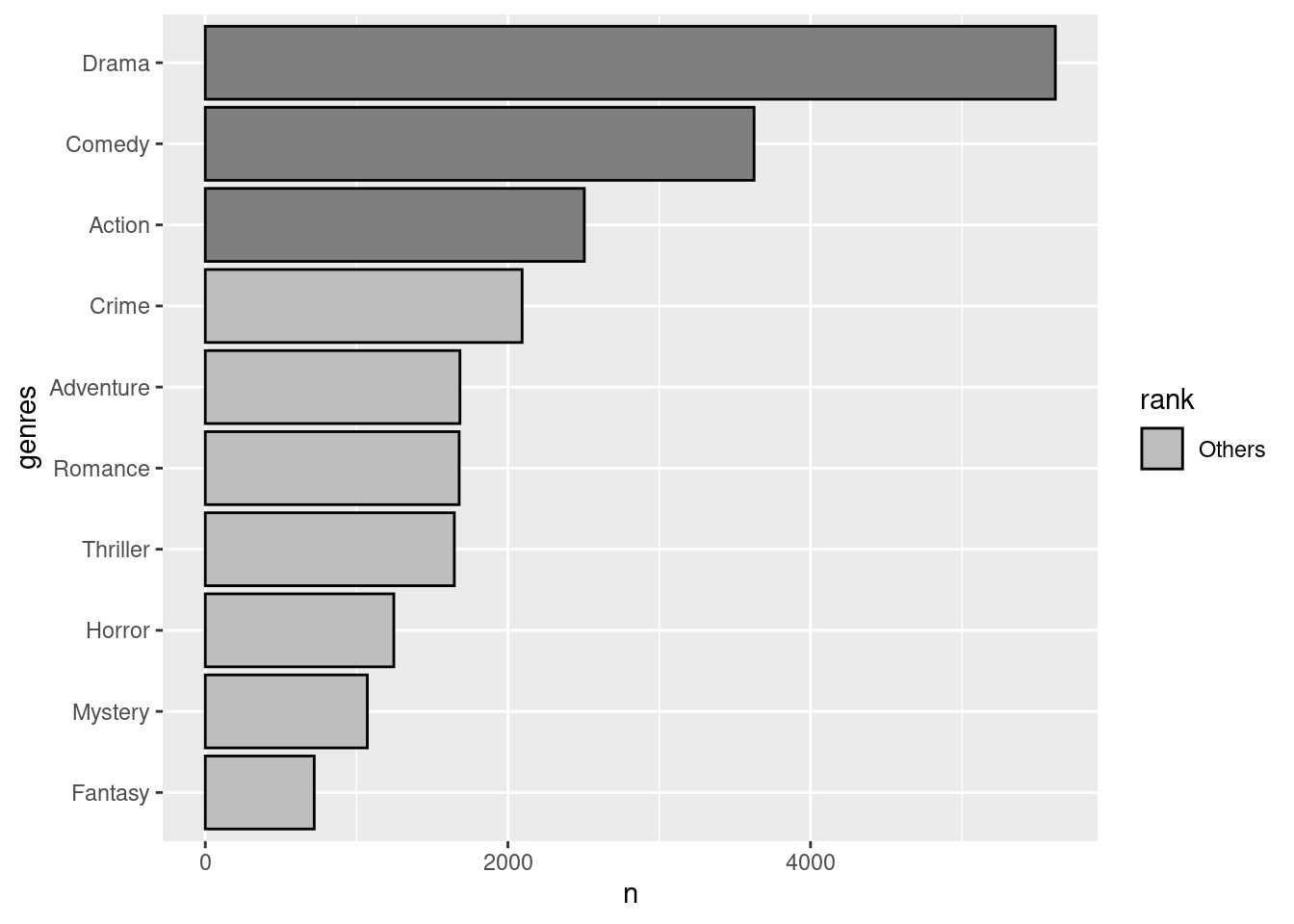
Most Common Individual Genres

df_unnested_genre |> 
  count(genres) |> 
  arrange(desc(n)) |> 
  slice_head(n = 10) |> 
  mutate(rank = if_else(row_number() <= 3, 'Top_3', 'Others')) |> 
  ggplot(aes(genres, n, fill = rank)) +
  geom_col() +
  scale_fill_manual(values = c('Top_' = '#FFA07A', 'Others' = 'grey')) +
  coord_flip()